Muon optimizer: qk-clipping, orthogonalization strategies, and behavorial insights.
The Muon optimizer, introduced by Keller Jordan and collaborators in 2024, represents a significant advancement in neural network optimization. Unlike traditional optimizers that treat all parameters equally, Muon specifically targets the hidden layers of neural networks through matrix orthogonalization. This approach has demonstrated notable improvements in training efficiency, achieving state-of-the-art performance in tasks such as CIFAR-10 speedrunning and NanoGPT training.
The motivation behind Muon stems from the need to address the inefficiencies observed in traditional optimization methods, particularly in the context of large-scale neural networks. Studies have shown that updates generated by standard optimizers like SGD-momentum and Adam often result in high-condition-number matrices, indicating low-rank updates dominated by a few directions. This can hinder effective learning, as it limits the exploration of diverse directions in the parameter space.
Muon tackles this issue by applying a Newton-Schulz iteration to orthogonalize the update matrices, effectively replacing them with the nearest semi-orthogonal matrices. This orthogonalization process increases the scale of “rare directions,” which, despite having small magnitudes in the update, are crucial for learning. By promoting a more balanced exploration of the parameter space, Muon enhances the optimizer’s ability to navigate complex loss surfaces, leading to improved generalization and performance
Furthermore, Muon’s design allows for efficient scaling to large models. Recent research has identified key techniques, such as adding weight decay and carefully adjusting the per-parameter update scale, that enable Muon to scale effectively without the need for extensive hyperparameter tuning. These advancements have facilitated the training of large-scale models, such as the Moonlight Mixture-of-Expert model, demonstrating Muon’s scalability and effectiveness in large-scale settings
Motivation
The motivation for this work is to explore the latest advances in neural network optimization and provide a practical, up-to-date implementation of the muon optimizer that incorporates these developments.
By developing muon-clip, an open source implementation of the muon optimizer featuring the latest research advancements, this work aims to enable reproducible experiments, offer insights into the inner workings of Muon, and make it easier to integrate Muon’s strategies into a variety of models.
QK-clipping
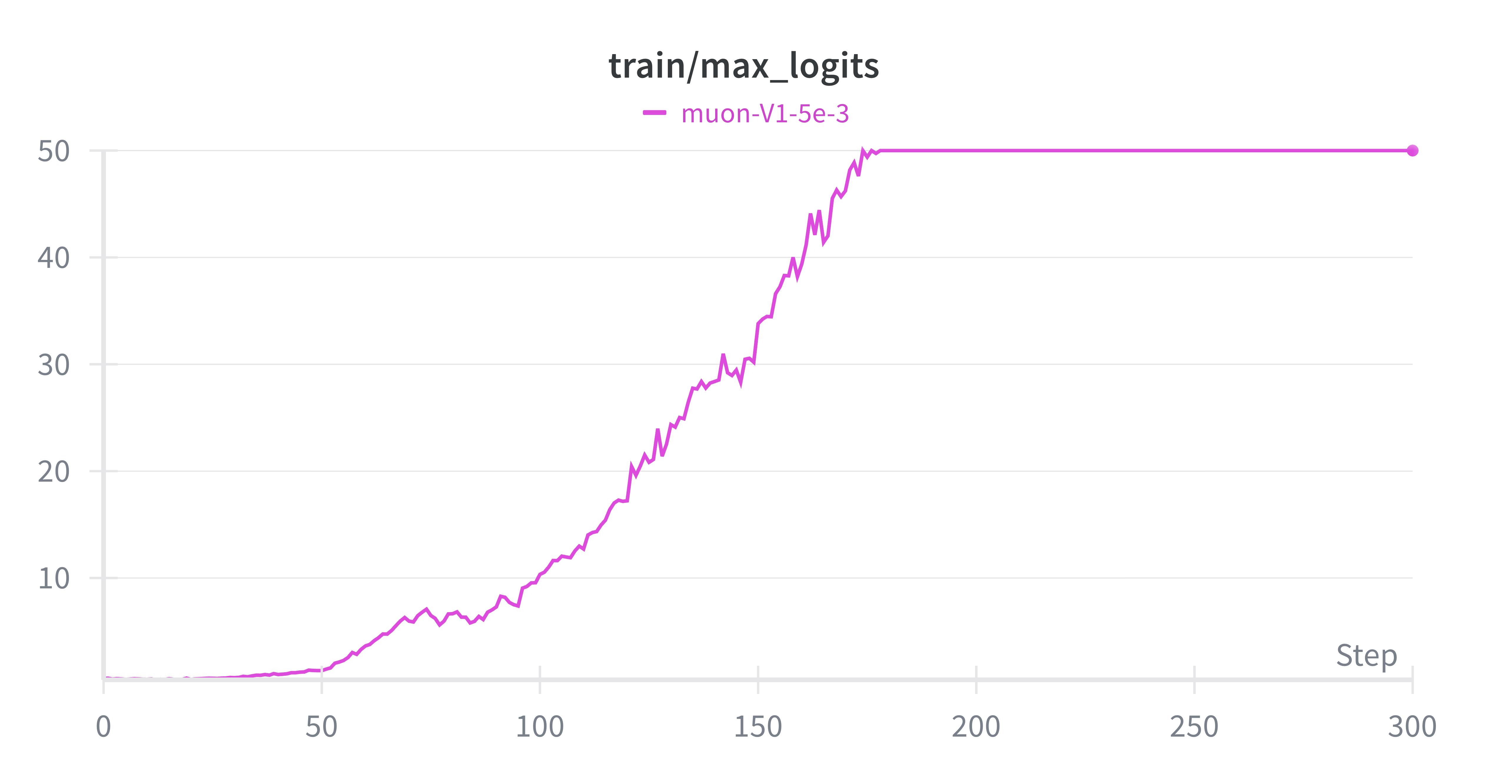
QK-Clipping is a method proposed by the Kimi K2 team to prevent a common issue in large language model training: attention logits explosion. Although this issue occurs more generally, it is especially problematic with Muon, because Muon’s updates allow the spectral norms of the query/key weight matrices to grow more freely (particularly at higher learning rates), which exacerbates the explosion of logits.
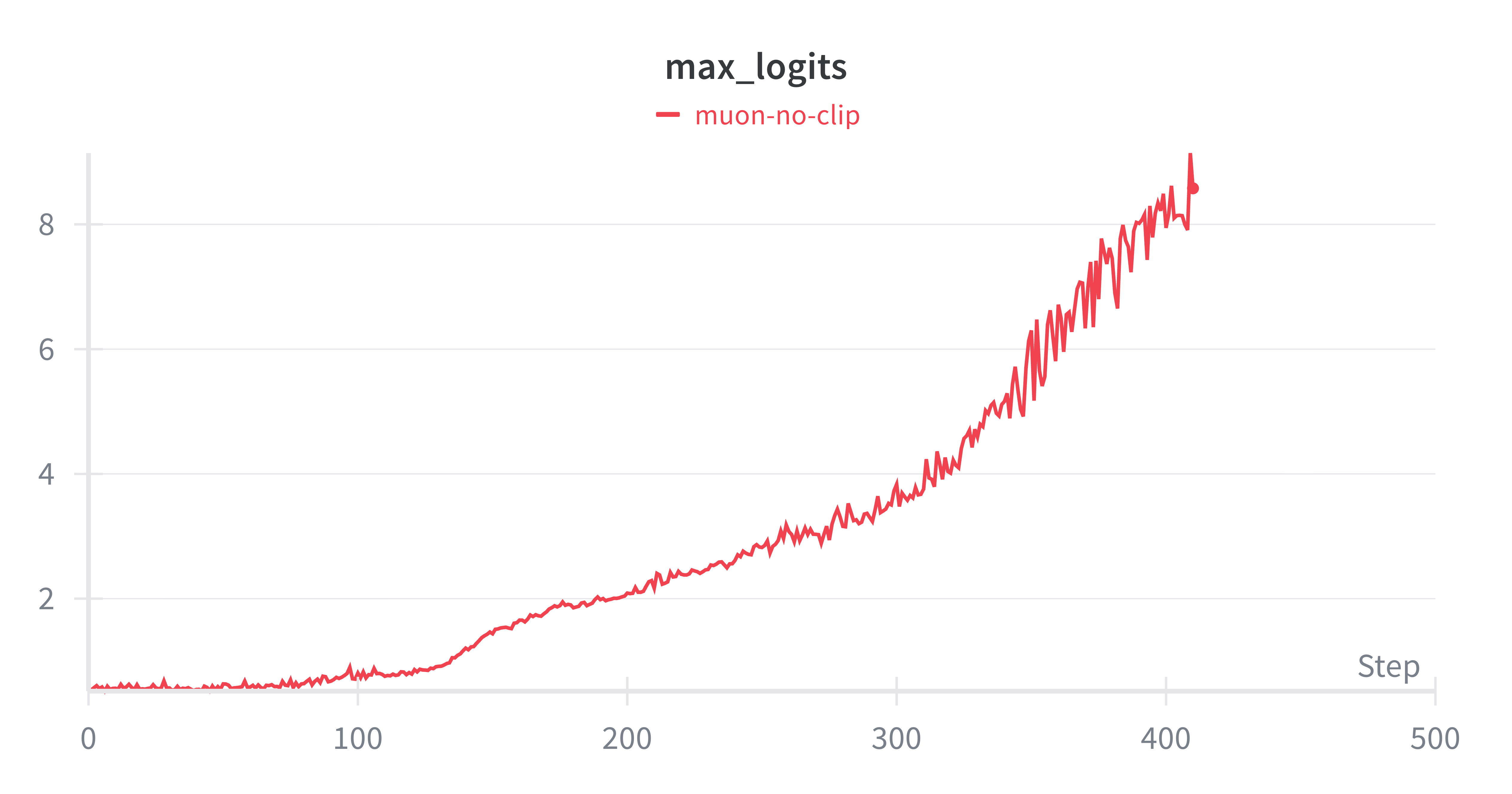
During training, attention logits are computed as the dot product between query (Q) and key (K) projections.
If the spectral norms of these matrices grow too large, the logits can explode, saturating the softmax function and halting learning. This is especially problematic in large-scale models, where instability can quickly derail training.
How QK-Clipping Works
QK-Clipping is an adaptive weight clipping mechanism applied to Q and K matrices:
- Monitor attention logits: During the forward pass, the maximum unnormalized logit is computed for each attention head.
- Compute scaling factor: If this maximum exceeds a predefined threshold (e.g., τ = 100), a scaling factor is calculated as for each head.
- Rescale Q and K weights: Both matrices are respectively multiplied by and , reducing the amplitude of the logits and stabilizing training.
This method allows logit control without changing the model architecture, making it a lightweight yet effective stabilization technique. In our experiments, we also show that this technique can even improve the convergence rate of small models (see experimentations result section).
Orthogonalization Strategies
This section explores different strategies to perform orthogonalization of matrices.
Singular Value Decomposition (SVD)
For any real matrix
there exists a factorization called the Singular Value Decomposition (SVD):
where:
- is an orthogonal matrix,
- is an orthogonal matrix,
- is a diagonal matrix containing the singular values.
The nearest orthogonal matrix (in Frobenius norm) to is given by:
This method is highly accurate, since it directly provides the best orthogonal approximation. However, computing the SVD is computationally expensive (complexity ), which makes it less practical for scenarios such as training deep neural networks, where repeated orthogonalization is required.
Newton–Schulz (NS) Orthogonalization
A widely used approach to matrix orthogonalization is the Newton–Schulz (NS) iteration, which iteratively refines an input matrix toward its nearest orthogonal factor.
Given a matrix (M), we first normalize it to control the spectral radius:
The iterative update takes the form:
where the coefficients ((a, b, c)) determine both convergence and stability.
With properly chosen coefficients, the iteration converges quadratically to the orthogonal polar factor of (M).
- Baseline coefficients:
corresponding to the classical 5th-order NS scheme.
- Muon-optimized coefficients:
which were empirically tuned in the Muon optimizer.
These yield a higher derivative at 0, accelerating the convergence of small singular values.
In practice, the original Muon implementation applies 5 iterations, which is sufficient to obtain an accurate approximation of the orthogonal matrix for deep learning applications. For more details, see Keller’s blog post.
Chebyshev-Accelerated Newton–Schulz (CANS) Iteration
Overview
The classical Newton–Schulz (NS) iteration is widely used for matrix orthogonalization because it relies only on matrix multiplications, making it efficient on modern hardware. However, its convergence speed is limited because the iteration coefficients are fixed and not adapted to the singular value distribution of the input matrix.
To address this, a Chebyshev-accelerated Newton–Schulz (CANS) method has been proposed (Ekaterina Grishina). It leverages Chebyshev-type polynomials and the alternance theorem to derive optimal coefficients that adapt to the spectrum of the matrix.
Key Ideas
-
Classical NS iteration:
Uses a fixed 5rd-order polynomial
Convergence requires specific spectral conditions and can be slow when singular values are widely spread. -
CANS method:
- Finds optimal odd polynomials that best approximate the unity function on the interval ([σ_{\min}, σ_{\max}]), where the singular values lie.
- Uses explicit formulas for degree-3 polynomials and the Remez algorithm for higher degrees.
- Allows construction of inexact orthogonalization polynomials confined to ([1 - δ, 1 + δ]), balancing accuracy and efficiency.
- Maximizes polynomial derivative near zero, which speeds convergence for small singular values.
Why CANS is More Accurate
-
Spectrum-adapted coefficients
Unlike classical NS with fixed coefficients, CANS tunes its polynomial coefficients to the actual singular value range, ensuring tighter error bounds. -
Quadratic error decay
The optimized scheme achieves faster convergence, with error shrinking roughly as (ε_{n+1} ≤ ε_n^2). -
Better control of approximation error
CANS allows explicit trade-offs between exact and approximate orthogonalization, which is especially useful in deep learning optimizers (e.g., Muon). -
Higher derivatives at zero
This design improves the rate at which small singular values move toward 1, leading to quicker stabilization of the spectrum.
Pseudo-code (simplified)
Input: Matrix M, number of iterations s, polynomial degree d

1. Normalize:
   X ← M / σ_max(M)             # Estimate largest singular value σ_max(M)

2. Initialize spectrum bounds:
   [a, b] ← [σ_min_est, 1]
  # If σ_min is unknown, use δ-orthogonalization:
  #   - Start from the interval [0, 2]
  #   - Iteratively apply the Remez algorithm
  #   - Push all singular values into [1 - δ, 1 + δ]
  # [a, b] ← [1 - δ, 1 + δ]

3. For i = 1 to s do:
      - Compute Chebyshev-optimal polynomial p_d,a,b(x)
        that best approximates 1 on [a, b] with remez algorithm
      - Update matrix:
        X ← p_d,a,b(X)
      - Update bounds:
        [a, b] ← [1 - ε, 1 + ε]   # ε = approximation error of polynomial

4. Return X  # Approximated orthogonal factor
For details on the evaluation of orthogonalization strategies, please refer to the experimental results section.
Behavorial insights: Understanding Muon Compared to Other Stochastic Optimizers
Gaining an intuition for what Muon brings compared to other stochastic optimizers, such as Adam, can be challenging. This section aims to provide some behavorial insights by visualizing how Muon behaves differently and what makes it a more exploratory and robust optimizer.
The code used for this part is available on GitHub: Understanding Muon.
A Simple Illustrative Problem
Consider a simple a function:
where each is a degree-2, 3-dimensional polynomial. Choosing three input and output dimensions allows us to easily visualize the model’s vector outputs in 3D.
We define our model as , with , and aim to solve:
where is the quadratic loss.
Concretely, the model consists of a linear layer (with or without bias i.e, n=9 or n=12) and a ReLU activation function (the ReLU nonlinearity is added to better mimic conditions of neural network training, even though the underlying target is polynomial). Our goal is to optimize this model for the problem above.
On Model Capacity
Note that the network described above is under-parameterized and mis-specified for the posed problem. The best solution, which would almost surely converge to zero, is the following model:
Here, the model directly learns the features of the three polynomials (i.e., the monomials of degree ≤ 2).
But the objective in this section is different: we intentionally place ourselves in realistic conditions. In practice, most non-convex optimization problems (e.g., deep learning, LLM training) are carried out on networks that are sub-optimal in architecture. They cannot perfectly represent the data distribution, either because they are under-parameterized (lacking sufficient capacity to represent the function) or mis-specified. This reflects real-world training scenarios much better than providing the exact optimal model.
Hypothesis: Why Muon Helps
Hypothesis regarding Muon:
When the network is under-parameterized/mis-specified (as is almost always the case in non-convex deep learning tasks1) and/or poorly conditioned (i.e regions of the parameter space where gradient propagation is weak or highly anisotropic2), Muon can retain exploration capacity, while Adam and other stochastic optimizers are constrained to explore only the directions that are analytically “easy” to access.
In other words:
- Adam and standard optimizers tend to align updates with dominant gradient directions, which in ill-conditioned networks means ignoring “rare” but important directions【Jordan et al., 2024】3.
- Muon, through its orthonormalization of updates, maintains update energy across multiple directions, enabling it to explore parts of the parameter space that Adam would under-utilize.
- This makes Muon especially effective on poorly conditioned networks, where conditioning problems cause slower convergence or loss of expressivity for other optimizers.
Experimental Setup
To test this idea, we compare performance under increasing levels of conditioning difficulty. Specifically, we test the following networks:
(calculer le condition number lambda max / lambda min)
Case 1
Case 2
Case 3
Case 4
These correspond to increasingly mis-specified/ poorly conditioned models for the problem:
- Case (1) is essentially linear and well-conditioned, but mis-specified.
- Cases (2) and (3) introduce ReLU nonlinearities, which not only create asymmetric gradient propagation but also truncate half of the input space (since negative polynomial values are mapped to zero). This deliberate loss of information increases the anisotropy of the optimization landscape, making the problem more poorly conditioned.
- Case (4) removes biases, further reducing flexibility and worsening conditioning.
Results
| Model | Adam test loss | Muon test loss | |
|---|---|---|---|
| 1.56 | 1.56 | 0.0 | |
| 1.19 | 1.14 | 0.05 | |
| 1.11 | 0.65 | 0.46 | |
| 2.03 | 0.89 | 1.14 |
We observe:
- On the well-conditioned linear case, Muon and Adam behave identically.
- As conditioning worsens (cases 2–4), Muon consistently outperforms Adam, with a substantial gap in the most poorly conditioned model (case 4).
This supports the hypothesis: Muon provides robust exploration under poor conditioning, while Adam is restricted to dominant gradient directions.
Note that all experiments were run with the same random seed to ensure faire comparison between muon and adam (same starting weights, train/test polynomial samples)
Visual interpretation and exploration measure
Below is a visualization of how the linear layer matrix evolves during training with Adam and Muon. Each color tracks represents one row of the linear layer, giving a view of how the optimizer explores directions within the 3D output space of the layer.


Even though it is visually apparent that Adam explores less in poorly conditioned cases, while Muon explores the space more extensively,
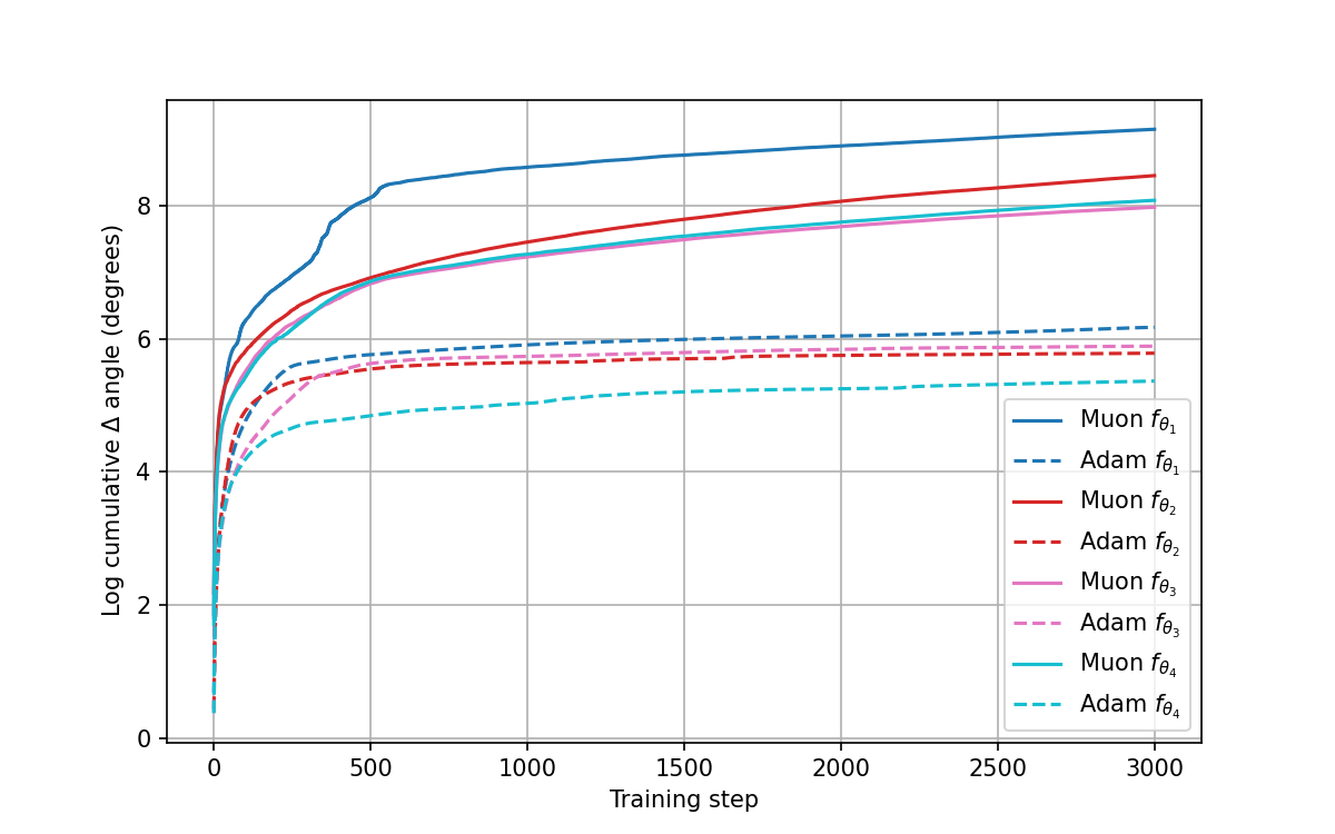
a more quantitative way to measure the amount of exploration is to compute the log cumulative angular deviation of each vector at each step, defined as:
Below is a representation of the through the steps for all 4 cases (higher values means more exploration):
Discussion of Results
The visualizations highlight a clear difference in the exploration behavior of Adam and Muon optimizers.
1.	Trajectory Space Exploration (Figure 1)
•	With Adam (left), trajectories remain confined to narrow subspaces, showing limited angular deviation between consecutive steps. This suggests that Adam tends to favor a more constrained path during training, which can reduce the optimizer’s ability to fully explore the parameter space.
•	In contrast, Muon (right) exhibits much broader trajectories across the space, with frequent and larger angular deviations. This indicates a more exploratory dynamic that allows Muon to probe different directions of the optimization landscape.
2.	Cumulative Angular Change (Figure 2)
•	The log cumulative difference of trajectory angles quantifies these observations. For all cases, Muon consistently accumulates larger angular changes than Adam, particularly in the early and middle stages of training.
•	This trend demonstrates that Muon maintains higher levels of exploration over time, while Adam rapidly converges to more stable, lower-variance trajectories.
•	Importantly, the gap is most pronounced for functions where the optimization landscape is less well-conditioned, reinforcing the idea that Muon is better suited to adapt to challenging geometries.
3.	Implications
•	The higher exploration of Muon could help avoid premature convergence and improve generalization by encouraging the optimizer to sample a broader range of solutions.
•	Adam’s more conservative trajectory might be advantageous in smooth, well-conditioned settings, but it risks stagnation when the landscape is complex or highly anisotropic.
Experimentations
Experimental Protocol
The experiments were designed with two main objectives:
1.	Verify the relevance of QK-Clipping as a stabilization technique when training with Muon.
2.	Compare orthogonalization strategies within Muon: the classical Newton–Schulz (NS, Muon-V1) versus the spectrum-adapted Chebyshev-Accelerated Newton–Schulz (CANS, Muon-V2).
To better highlight the differences between clipped and unclipped training, we deliberately used a high learning rate. This setup causes the logits to grow rapidly, which makes instabilities appear much earlier and thus accentuates the contrast between runs with and without QK-Clipping.
The evaluation followed two complementary steps:
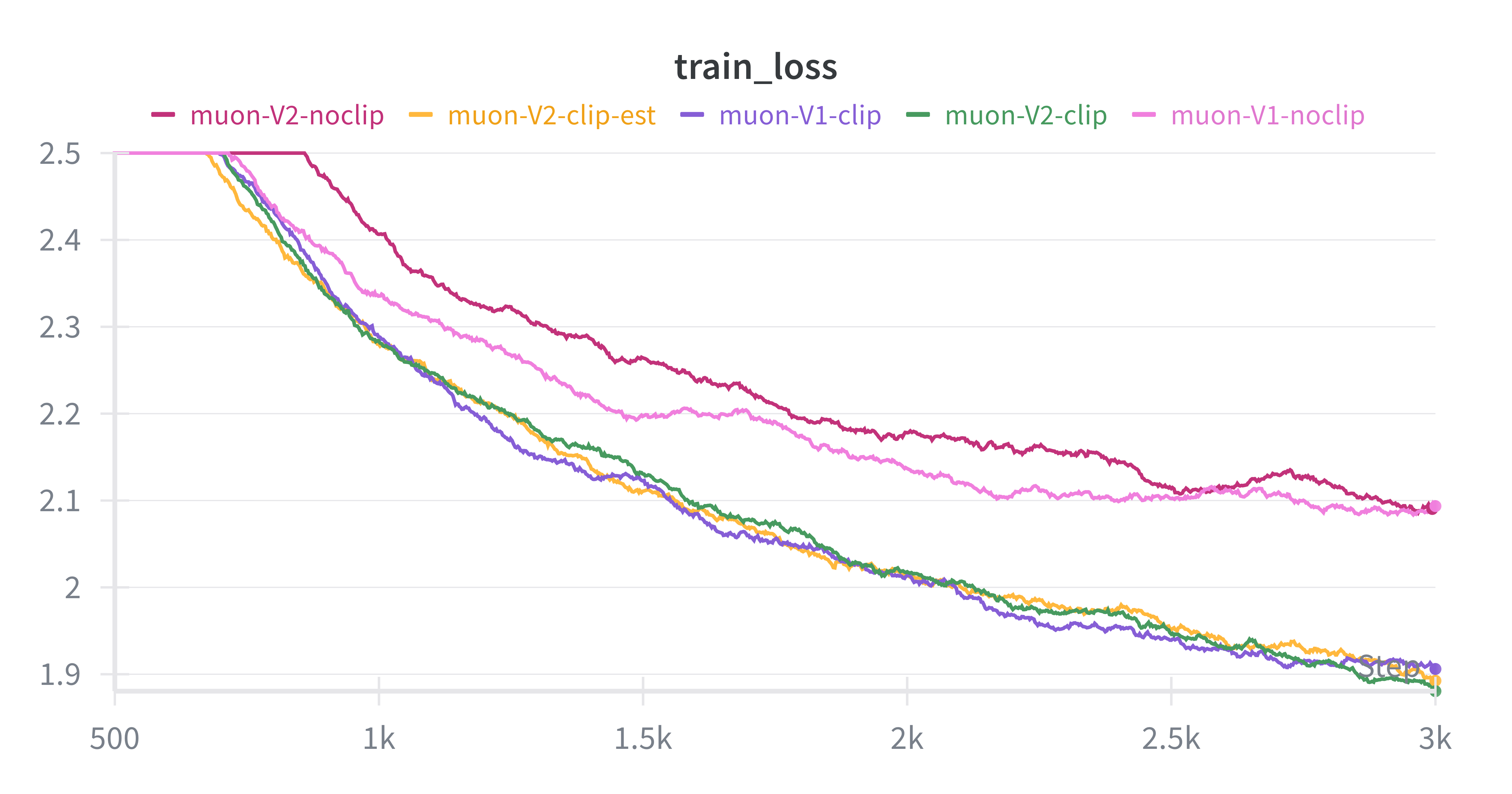
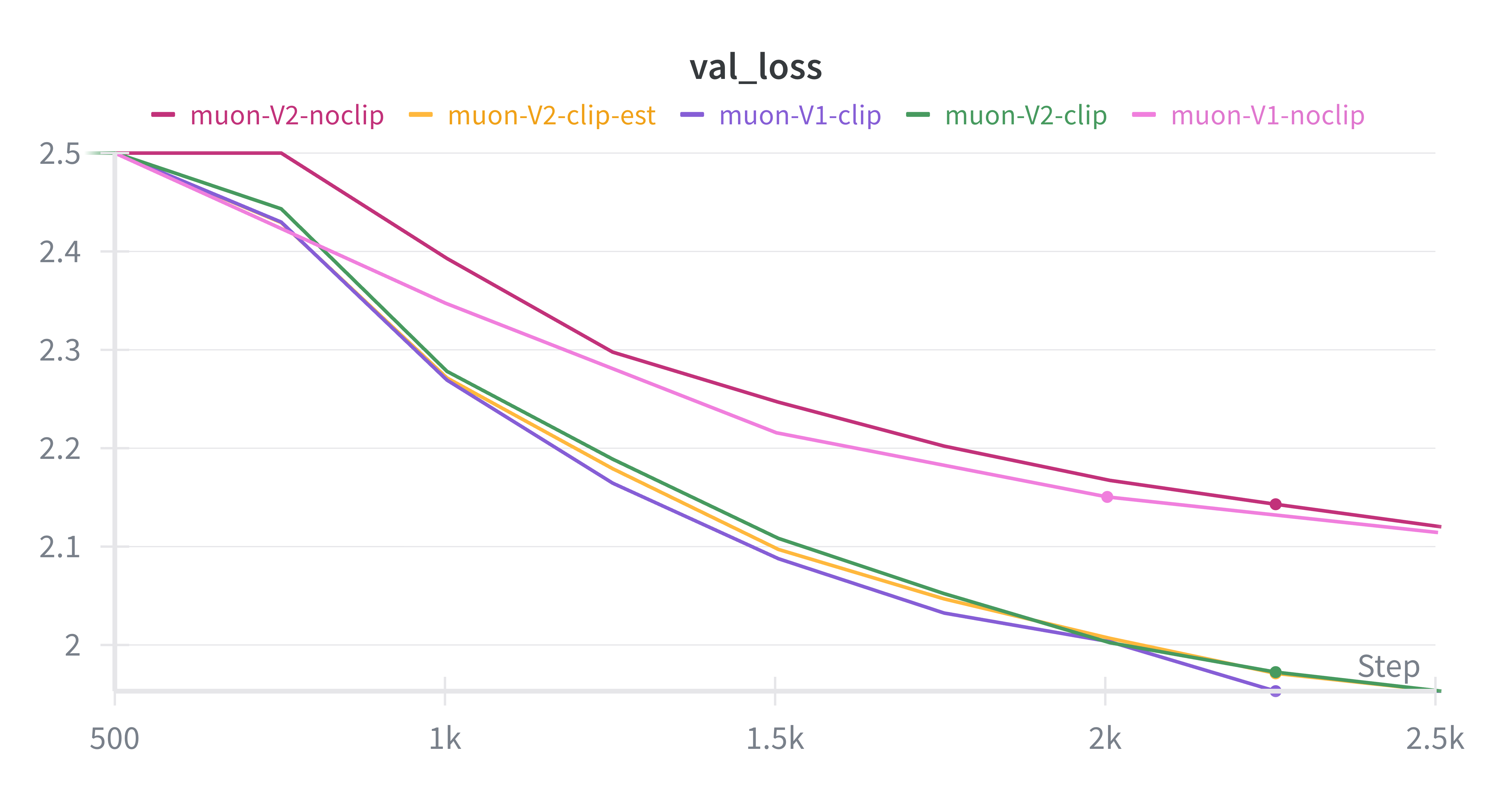
•	Step 1: Observe the training dynamics (train loss curves) under both clipping and orthogonalization choices.
•	Step 2: Validate these observations on the synthetic test problems from the Behavioral Insights section, covering a spectrum from well-conditioned to severely ill-conditioned tasks.
The test belows were realised with Le Carnet.
Discussion
From the curves we observe:
•	Without clipping (noclip): training rapidly stalls, with losses plateauing at higher values for both NS and CANS. This confirms that uncontrolled logit growth destabilizes optimization.
•	With QK-Clipping (clip / clip-est): training becomes stable, with losses steadily decreasing. Both NS and CANS benefit from clipping, but Muon-V1 (NS) consistently achieves slightly lower losses.
•	Overall: QK-Clipping proves to be essential for stable convergence, while NS remains the more reliable orthogonalization method compared to CANS.
Validation on Toy Models (table)
To further validate these findings, we evaluated Muon with NS and CANS on the four synthetic models defined earlier (Cases 1–4), which cover a spectrum from well-conditioned to severely ill-conditioned.
| Model | Muon NS test loss | Muon CANS test loss |
|---|---|---|
| 1.56 | 1.52 | |
| 1.14 | 1.32 | |
| 0.66 | 0.95 | |
| 0.89 | 0.84 |
The results confirm the trends observed in the plots:
•	NS (V1) generally outperforms CANS (V2), particularly in moderately conditioned settings (Cases 2 and 3).
•	Only in the most constrained setup (Case 4) does CANS slightly edge out NS, but overall the traditional NS method remains the more effective and consistent choice.
Conclusion
The experiments confirm that the Muon optimizer brings a clear advantage over classical optimizers like Adam in poorly conditioned or mis-specified settings. By orthogonalizing updates, Muon is able to maintain exploration in directions that Adam tends to ignore, leading to significantly better convergence and generalization when the optimization landscape is challenging.
However, regarding orthogonalization strategies, our results show that the Chebyshev-Accelerated Newton–Schulz (CANS) method did not prove to be more effective than the traditional Newton–Schulz (NS) scheme in practice. While CANS is theoretically appealing due to its spectrum-adapted coefficients, in our experiments the classical NS iteration remained at least as effective, and often more stable.
This suggests that, for now, NS orthogonalization remains the preferred approach for Muon, while CANS might require further refinements or more specific conditions to demonstrate its advantages.
References
- Keller Jordan, Yuchen Jin, Vlado Boza, Jiacheng You, Franz Cesista, Laker Newhouse, Jeremy Bernstein. “Muon: An optimizer for hidden layers in neural networks”. Accessed 06.09.2025, URL: https://kellerjordan.github.io/posts/muon/ (2024)
- Ekaterina Grishina, Matvey Smirnov, Maxim Rakhuba.”Accelerating Newton-Schulz Iteration for Orthogonalization via Chebyshev-type Polynomials”. arXiv preprint arXiv:2506.10935 (2025)
- Kimi team.”KIMI K2: OPEN AGENTIC INTELLIGENCE”. arXiv preprint arXiv:2507.20534v1 (2025)
- Jingyuan Liu et al. “MUON IS SCALABLE FOR LLM TRAINING”. arXiv preprint arXiv:2502.16982 (2025)
Citation
@misc{sinoue2025muon,
  title   = {Muon optimizer: qk-clipping, orthogonalization strategies, and behavorial insights.},
  author  = {Sinoué GAD},
  year    = {2025},
  howpublished = {},
  note    = {An implementation of the muon optimizer featuring the latest research advancements and some insights towards behavorial insights.}
}
Footnotes
-
Simsek et al. (2023) formalize the under-parameterized regime as when a “student” network with hidden neurons attempts to approximate a “teacher” network with neurons. ↩
-
See Sutskever et al. (2013), “On the importance of initialization and momentum in deep learning,” on how poor conditioning slows gradient descent. ↩
-
Jordan et al. (2024) show that gradient updates in Adam/SGD often have nearly low-rank structure, dominated by a few directions. Muon orthogonalizes these updates to amplify rare but important directions. ↩